Getting started

Let's assume you took the following image img, reshaped it to WHCN format (width, height, color channels, batch dimension) and ran it through a vision model:

using Images
img = load(joinpath(asset_dir, "img1.png")) # load image file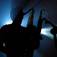

You might use an input space attribution method (for example from ExplainableAI.jl) to determine which parts of the input contributed most to the "saxophone" class.

Let's load such an attribution x in WHCN format:

x = load(data_heatmap, "x") # load precomputed array from file
typeof(x)

Array{Float32, 4}

size(x)

(224, 224, 3, 1)

To make this attribution more interpretable, we can visualize it as a heatmap:

using VisionHeatmaps
heatmap(x)

(a vector displayed as a row to save space)

By default, to support batched explanations, a vector of heatmaps is returned. Since our following examples don't use batches, we will use the only function to unpack singleton heatmaps:

using VisionHeatmaps
heatmap(x) |> only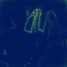

Custom heatmapping pipelines

VisionHeatmaps internally applies a sequence of image transformations in what we call a Pipeline. The default pipeline corresponds to:

pipe = NormPooling() |> ExtremaNormalization() |> Colormap()

Pipeline(
  NormPooling(),
  ExtremaNormalization(),
  Colormap(:batlow),
)

We can apply this pipeline by passing it to heatmap:

heatmap(x, pipe) |> only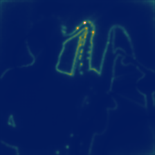

Image orientation

heatmap assumes WHCN input and flips the width and height dimensions by default, so that pipelines return display-oriented images. Because of this, pipelines don't need to include FlipImage. It remains available for pipelines that operate on already-oriented arrays.

In the following subsection, we will explain and modify this pipeline step by step.

Attribution pooling

For arrays with multiple color channels, the channels need to be reduced to a single scalar value for each pixel, which is later mapped onto a colormap.

For this purpose, pipelines use the attribution pooling functions from XAIBase.jl. Let's compare the two most commonly used ones. NormPooling reduces color channels in the array by taking their norm, whereas SumPooling takes the sum:

pipe = NormPooling() |> ExtremaNormalization() |> Colormap()
heatmap(x, pipe) |> only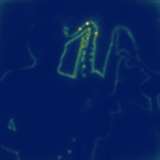

pipe = SumPooling() |> ExtremaNormalization() |> Colormap()
heatmap(x, pipe) |> only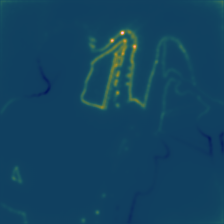

Normalization and colormaps

To map the now pooled array onto a colormap, we first need to normalize all values to the range $[0, 1]$.

For this purpose, two normalization functions are available:

ExtremaNormalization: maps the minimum and maximum value in the array onto $[0, 1]$.
CenteredNormalization: maps the negative and positive maximum absolute value of the array onto $[0, 1]$. Values of zero will be mapped to the center of the colormap.

A Colormap is then applied to the normalized values.

Since NormPooling only yields positive values, it is well suited for ExtremaNormalization and a sequential colormap like the default :batlow. SumPooling on the other hand can yield positive and negative values. If zero-values are meaningful, using CenteredNormalization with a divergent colormap like :berlin can be the right choice:

pipe = NormPooling() |> ExtremaNormalization() |> Colormap()
heatmap(x, pipe) |> only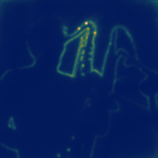

pipe = SumPooling() |> CenteredNormalization() |> Colormap(:berlin)
heatmap(x, pipe) |> only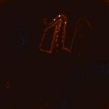

Heatmapping XAIBase attributions

When heatmapping an Attribution from XAIBase.jl, the default pipeline follows from its pooling function. Unsigned pooling functions like NormPooling use ExtremaNormalization and :batlow, whereas signed pooling functions like SumPooling use CenteredNormalization and :berlin. Use VisionHeatmaps.default_pipeline to inspect or modify the default pipeline.

Outlier removal

While this isn't part of the default heatmapping pipelines, previous heatmaps visibly emphasized three "dots" on the neck of the saxophone. Very high values in explanations tend to desaturate colors. For this purpose, we provide the adaptive PercentileClip. By default, it clips the 0.1-th and 99.9-th percentiles of values.

pipe = SumPooling() |> PercentileClip() |> CenteredNormalization() |> Colormap(:berlin)
heatmap(x, pipe) |> only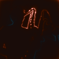

Custom colormaps

We can use any colormap from ColorSchemes.jl:

using ColorSchemes
pipe = NormPooling() |> ExtremaNormalization() |> Colormap(:jet)
heatmap(x, pipe) |> only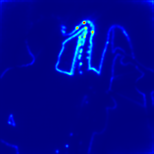

pipe = NormPooling() |> ExtremaNormalization() |> Colormap(:viridis)
heatmap(x, pipe) |> only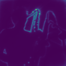

We strongly suggest to only use sequential colormaps with ExtremaNormalization and divergent colormaps with CenteredNormalization.

ColorSchemes.jl catalogue

Refer to the ColorSchemes.jl catalogue for a gallery of available colormaps.

Overlays

Singleton heatmaps can be overlaid on top of the original image. This can be used to recreate CAM-like heatmaps (usually in combination with ResizeToImage):

pipe = NormPooling() |> PercentileClip() |> ExtremaNormalization() |> Colormap(:jet) |> AlphaOverlay()
heatmap(x, img, pipe) |> only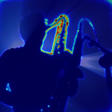

Heatmapping batches

heatmap can also be used to visualize input batches. Let's assume we computed an input space attribution batch for the following images.

imgs = [load(joinpath(asset_dir, f)) for f in ("img1.png", "img2.png", "img3.png", "img4.png", "img5.png")] # load image files

(a vector displayed as a row to save space)

Once again, we assume that batch is in WHCN format:

batch = load(data_heatmaps, "x") # load precomputed array from file
typeof(batch)

Array{Float32, 4}

size(batch)

(224, 224, 3, 5)

Calling heatmap will automatically return an vector of images:

heatmap(batch)

(a vector displayed as a row to save space)

These heatmaps can be customized as usual:

pipe = SumPooling() |> CenteredNormalization() |> Colormap(:berlin)
heatmap(batch, pipe)

(a vector displayed as a row to save space)

By default, each heatmap in a batch is normalized individually, so colors can't be compared across heatmaps. Wrapping the normalization in a BatchedNormalization normalizes the whole batch to a shared value range instead:

pipe = SumPooling() |> BatchedNormalization(CenteredNormalization()) |> Colormap(:berlin)
heatmap(batch, pipe)

(a vector displayed as a row to save space)